Learning Resources

Lesson

There are no new concepts presented in this lesson. It is a matter of applying what you learned about regression analysis in the last lesson to some real world problems. Specifically, the stopping distances of an automobile under various speeds and road conditions are analyzed.

One of the road conditions, gravel, is done as an example to help you with the rest. The table for stopping distances on gravel is reproduced below.

speed	0	10	20	30	40	50	60	70	80	90	100
dist.	0.00	0.78	3.14	7.08	12.59	19.68

The entire problem can be done using the TI83 calculator. Recall the steps:

1. Enter the data in lists.
2. Do a scatter plot to see the "basic shape" of the data.
3. Check the sequence of differences to confirm what the scatter plot suggests.
4. Do the appropriate regression.
5. Write the equation.

The final answer on the calculator is shown below:

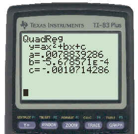
To see the major keystrokes necessary to get this solution click here.

Note: -5.67E-4 means -5.67 x 10^-4 which is 0.000567. Rounding the values of a, b, and c the equation is:
y = .0079x² - .00057x - .0011

Activity

1. Read through Focus B on pages 17 & 18 in your text.
2. Complete Focus Questions 10 - 16 on page 19
3. Do CYU Question 17

When you have completed these questions, ask your on-site teacher to get the solutions for you from the Teacher's Resource Binder and check them against your answers. After you do this, if there is something you had trouble with and still do not understand, contact your on-line teacher for help.

After you do the assigned activities, click on the Test Yourself button at the top of the page for a quick quiz on this lesson.

Test Yourself

An automobile is tested for braking distances at various speeds with the following results:

Speed(km/h)	Distance(m)
0	0
50	24.15
80	53.07
100	75.61
120	97.18

Create a scatter plot and use the proper regression to find a possible equation to model this data.

Solution