Learning Resources

Lesson

The main outcome of this lesson is to be able to determine the equation of the curve of best fit for a set of data. The data may be what you have collected yourself, as is suggested in Investigation 3, or it may be data that someone else provides for you.

Regardless of where the data comes from, we will use technology (TI83) to do a regression analysis of the data and determine the equation of the curve of best fit. The reason we use technology to do the regression is because to do it by hand is a lengthy and very tedious process.

To be able to tell the technology which type of regression to do, we will look at a scatter plot of the data and determine if it "looks" linear, quadratic, cubic, etc. We will also use the sequence of differences to help determine if the data is linear, quadratic, cubic, etc.

If you have the necessary equipment you should conduct Investigation 3 and collect your own data. It makes the rest of the work much more meaningful. If at all possible, you should work with a partner to complete this investigation. To do the investigation you will need the following materials

• toy car or ball
• board or eaves trough - eaves trough preferable because it will prevent the object falling off the sides.
• a measuring device such as Calculator-Based Ranger^TM
• TI83 calculator

This is an excellent investigation for you if you are also doing physics. Check with your physics teacher as the materials required, especially a device like the Calculator-Based Ranger^? , may be available in one of the science labs. Also, you may be able to use this data for one of your physics labs. Conversely, you may be able to use the data from one of your physics labs for this investigation.

If you have the necessary materials, stop now and complete Investigation 3 on page 15 of your text before you go on to the next page. If you are not able to do the Investigation you can proceed directly to the next page.

We wish to find a function that describes a particular set of data. Our first step in the process is to graph the points on a grid and "eyeball" them to see if they look like any of the functions that we have studied. The main "shapes" we will be looking for will be restricted to linear, quadratic, and cubic. These are shown below just as a reminder to you.

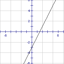
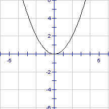
Linear Quadratic

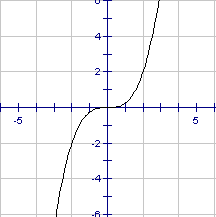
Cubic

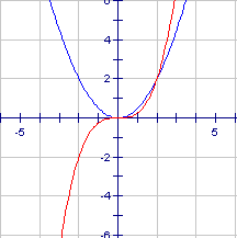
In these graphs, note the great similarity between the quadratic and cubic over part of the domain from 0 to 4. Both are drawn on the same axis below to emphasize this. It is something we have to be aware of when we are trying to pick the right curve to "fit to the data". If we have only a small few points we could quite easily mistake which function to use.

We will now find the "equation of best fit: for the data in the table below, which is from an experiment similar to the one suggested for Investigation 3. The time is measured in seconds and the distance from the recording device is measured in millimetres.

Time	0	0.2	0.4	0.6	0.8	1.0	1.2	1.4	1.6	1.8	2
Dist	1000	838	712	621	564	543	557	606	689	806	958

You can use grid paper and plot the points as shown in the interactive below:

On the next page you will see how to use the TI83 to accomplish the same end.

Instead of using graph paper, we can use our TI83 to plot the points for us. Since we will be using the TI83 to do the regression and this will require entering the data in two lists, we may as well use it to plot the points as well. The resulting plot of the data points from our table is shown below:

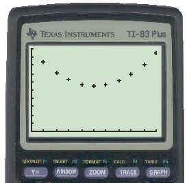
To see the key strokes necessary to get this plot click here. That is the method you can use to enter the data and plot the points for the problems that will be assigned in the text book.

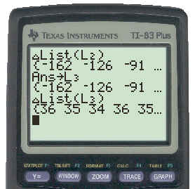
The reason we wanted this plot was to determine what type of function would best describe the data in the table. The points look very much like the shape of a quadratic, so we could proceed directly to do a quadratic regression. However, to be more positive that the data is quadratic we will check the sequence of differences. Again, the calculator can be used to do this for us and the result of that is shown below.

To see the key strokes necessary to get this click here.

The second level differences are not exactly equal. In fact, differences at any level which are obtained from experimental data are rarely, if ever, exactly equal. This is because of the errors in the initial measurements used to obtain the data. However, if the differences are "close enough" they "suggest" the type of relation under consideration.

We now have two indications that the data in our original table is quadratic in nature. The scatter plot "looked" quadratic and the sequence of second level differences was "almost" common. It is now only a matter of using the calculator to do a quadratic regression to determine the equation for us.

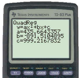
The equation will have the form y = ax² + bx + c and the calculator will calculate the values of a, b, and c for this particular set of data. Remember that we entered the time in list L₁ and the distance in list L₂. The result of the regression is shown below:

To see the key strokes necessary to get this click here.

The equation that describes the data in our initial table (with the coefficients rounded to the nearest whole number) is:

y = 436x² - 892x + 999

If you look at the equation developed by the calculator and substitute x = 0 into it, then you find that y = 999. However, if you look at the table, when x = 0 you find that y = 1000. The equation is not an "exact" description of the table. This occurs because the values in the table came from experimental results and contain measurement errors. What the calculator finds is the equation of "best fit" for all the data.

The steps necessary for finding the equation of best fit are summarized on the next page.

Summary

1. After performing an experiment or when data has been provided for you, organize it in table form.
2. Enter the data into the TI83 in two lists.
3. Use your TI83 to make a scatter plot of the data and see if it "looks" linear, quadratic, etc.
4. Use your TI83 to calculate the sequence of differences to see if it substantiates the initial decision you made by looking at the scatter plot.
5. Use your TI83 to do the appropriate regression on the data.

Now go to the top of the page and click on the Activities button.

Activity

• If you have not already done so and if you have the necessary materials, complete Investigation 3 on page 15 of your text.
• If you do not do the experiment yourself, ask your on-site teacher to get the Blackline Master 1.2.1 from the Teacher's Resource Binder and use the data in it to answer the questions in Investigation 3 on page 15.
• Complete Investigation Questions 1 to 4 on pages 15 & 16.
• Do the CYU Questions 5 -7, 8(a), 9

When you have completed these questions, ask your on-site teacher to get the solutions for you from the Teacher's Resource Binder and check them against your answers. After you do this, if there is something you had trouble with and still do not understand, contact your on-line teacher for help.

After you do the assigned activities, continue on to the Test Yourself section below for a quick quiz on this lesson.

Test Yourself

Find the equation of the curve of best fit for the data in the table below:

x	1	2	3	4	5	6
y	3.536	2.176	1.616	1.856	2.896	4.736

Solution