
Learning Resources
Lesson
In this lesson we are going to explore experimental probability by performing simulations to model some situations. A simulation is a model that is usually simpler to work with than the situation you wish to explore. We have to be careful that the simulation model matches the original situation as closely as possible. Otherwise the simulation results may not be a true reflection of the situation.
It will be possible to calculate the theoretical probability of the situations we will explore in this lesson. We then want to compare this theoretical probability with the results of the simulation which will give us the experimental probability.
In Step A , you should see readily what the theoretical probability will be since there are five equally likely outcomes and only one of them involves guessing correctly.
Step B and Step C requires you to state the problems variables and any assumptions you have to make during the simulation. For Step D, the simulation can be performed in a number of ways (recall the simulations done in earlier courses with respect to statistics); putting five coloured marbles or five numbered pieces of paper in a bag and drawing one; spinning a spinner made from a circle with five equal sectors marked on it; using technology such as a calculator to pick one of five random numbers.
As you perform the trials for Step E expect large fluctuations from your expected values from Step A after 5 trials. As your number of trials increase, it should become closer to the expected value. Note in the table that the experimental probability is cumulative with each group of five trials. Keep your data organized since you should pool your results with the rest of the class after the investigation is complete.
The graph is Step F will be a broken line graph; the theoretical probability a simple horizontal line. It should be obvious from the graph how the theoretical probability and experimental probability are related as the number of trials increase.
Example 1
Run a simulation to determine the experimental probability of the following situation. You are a bomb disposal expert trying to diffuse a bomb. When the cover is removed there are six wires attached to the detonator. Cutting one of the wires will diffuse the bomb, cutting any of the other five will detonate it. If you have no idea which wire to cut, what is the probability you will successfully diffuse the bomb by randomly selecting a wire to cut?
Solution
The theoretical probability is straight forward. There are six possible outcomes only one of which favours success. Thus the theoretical probability is:
![]()
Determining the experimental probability by doing trials with the actual situation is really not a desirable option, we will set up a simulation. Any model that will give us six events, all of which are equally likely to occur, will serve our purposes. Some examples might be: rolling a six sided die; putting six coloured marbles or six numbered pieces of paper in a bag and drawing one; spinning a spinner made from a circle with six equal sectors marked on it; using technology such as a calculator to pick one of six random numbers.
For this simulation let's use the TI83 to randomly select an integer from 1 to 6. We can pick any one of the integers from 1 to 6 to represent "success" and the other five integers will represent failure. Let's use 2 to represent success. If we run the simulation 5 times on our calculator we get:
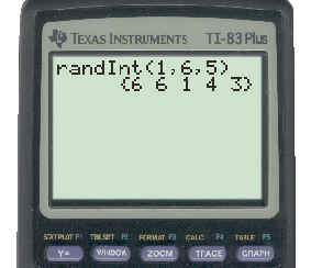
This is equivalent to a simulation of putting 6 pieces of paper with the integers 1 to 6 on them in a hat and drawing out one at a time, recording it, replacing it in the hat, and drawing again. The first time you drew a 6, the second time another 6, the third time a 1, the fourth time a 4, and the fifth time a 3. To see the TI-83 keystrokes necessary to get this result click here.
In our five trials the integer 2, which represented success, did not appear. The number of "successful" trials was 0 and the probability of success is:
![]()
This is clearly not the same as what was expected since the theoretical probability was ![]() .
.
We can repeat the simulation using as many trials as we like. For example if we do the simulation with 25 trials we get:
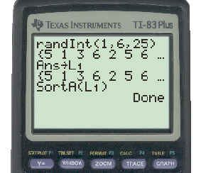
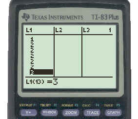
The results of the 25 trials have been stored in list L1 and sorted for easy counting. A display of results in list form is shown below:
To see the TI83 keystrokes necessary to get this result click here.
In our twenty five trials the integer 2, which represented success, appeared 5 times. The number of "successful" trials was 5 and the probability of success is:
![]()
Again this is not the same as the theoretical probability.
We could complete the simulation with more trials and compare that to the theoretical probability. However, that is what you are asked to do in a very similar problem in Investigation 1 in you text.
You don't have to use the calculator to do the simulation in Investigation 1. You can use any of the other methods suggested above. However, the calculator gives the trial results much quicker.
Investigation 2 continues the work on experimental probability and how to use simulations to determine them. Open your text to page 304 and read through the Investigation. The investigation deals with the probability of two people meeting each other under certain conditions. This problem, at this stage, must be viewed experimentally through a simulation; you will revisit it later in the unit in a theoretical way.
For Step A and Step B you only need to restate the problem in your own words. Since there are two times involved, your simulation must involve two separate trials one for each person and determine whether the times result in a meeting. The assumption of Step C is that there will be no overlap that would occur in the real world - either they meet within the ten minutes or not; for example after exactly 10 minutes, there is still a chance they could meet either coming or going from the DMV.
For Step D you need to set up a simulation that will select a time for Alyssa between 10:00 and 10:30 and also select a time for Ja-Wen between 10:00 and 10:30. If the two times are 10 min or less apart they meet. If the two times are greater than 10 min apart they do not meet.
Suggestion 1
One simple simulation would be to use two bags (boxes, hats, etc.), one for each person. In each bag put pieces of paper with the times on it, e.g. 10:00, 10:01, 10:02, .....,10:29, 10:30. Draw one piece of paper from each bag and record the results in a table similar to the one on page 305 of your text. Compare the two times and decide if they meet. Replace the pieces of paper, shake the bag, and repeat the process 50 times.
Suggestion 2
You could also use your TI-83 calculator to simulate this problem. Use it as you did in the example. This time you want to select 2 random integers between 0 (representing 10:00) and 30 (representing10:30). If the difference between the two random integers is 10 or less, the people meet, otherwise they don't. One result of this is shown below:
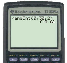
In the trial above, we interpret the simulation result (19 , 6) as meaning Alyssa arrived at 10:19 and Ja-Wen arrived at 10:06. That means they did not meet each other. Use your calculator to repeat this 50 times and record your results in a table similar to the one on page 305 in your text. To see the key strokes necessary to perform this simulation click here.
Suggestion 3
If you use the TI-83 as described above, you will have to repeat the process 50 times. One way of getting around this is to pick the 50 random numbers representing the 50 possibilities for Alyssa's arrival time and store them in a list. Then do the same for Ja-Wen's arrival times. Compare the corresponding numbers in the lists to see if they "meet". One result is shown below:
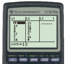
The first pair (18, 24) indicate they will meet as the difference is less than 10. The third pair (6, 18) indicate they will not meet as the difference is greater than 10. To see the key strokes necessary to perform this simulation click here. It is possible to arrange the differences on the TI-83 to simply count the number of values 10or less. Click here for a demonstration.
Suggestion 4
If you are familiar with the use of spreadsheets such as Microsoft Excel, you can use them to very quickly generate a series of random numbers to simulate this problem.
Caution: The random number generator in Excel works differently than in the TI-83. In Excel the function returns a decimal quantity between 0 and 1. To turn the result into integers you have to multiply by the upper limit of the integers you wish to choose and then round the decimal quantity to the integer below it.
A spreadsheet can do much more than simply generate a series of random numbers. In our problem, it can also be "programmed" to tell if the results of a trial mean they meet or not. It can also count the number of times the meeting occurs, and it can return the probability by dividing the number of successful trials by the total number of trials.
The following spreadsheet is set up to do 50 trials each time the simulation is run. By changing the number of the simulation in cell C1, the spreadsheet re-calculates 50 pairs of random numbers, checks to see if they differ by 10, counts the number of "yes" responses, and calculates the probability. You have to scroll down to row 52 to see the answer. You can use the results to help answer Step G in Investigation 1 on page 305. Enter a different simulation number and see how the probability changes.
For the last three steps, Steps E, F, and G, record your results as indicat4ed and compare to other people in your class; pool your results if possible to find a better solution. By comparing your results, you should immediately find that the experimental probabilities are going to differ; however, you should be able to come up with a reasonable answer.
You should now be ready to do the work in your textbook related to using simulations to find experimental probability.
You should have access to the TI-83 calculator and that may be the best method to use for simulation as most events can be modeled using some form of random numbers. If you are comfortable with, and have access to spreadsheets, you have a fast and convenient way of doing many repetitions of the same simulation and/or doing many trials in each simulation. Without one of these pieces of technology, you have to rely on selecting objects (pieces of paper, marbles, etc.) from bags or hats, or tossing dice of some kind.
Activity
Investigation 1 Questions p.304. Complete 12 and 13
Check Your Understanding p.305 - 306. Complete 14, 15 and 16
When you have completed these questions, ask your on-site teacher to get the solutions for you from the Teacher's Resource Binder and check them against your answers. After you do this, if there is something you had trouble with and still do not understand, contact your on-line teacher for help.
After you do the assigned activities, continue on to the Test Yourself section below for a quick quiz on this lesson.
Test Yourself
- Is it possible that the experimental probability found by doing a simulation will be exactly equal to the theoretical probability? Explain with an example. Write this in your Journal.
- Based on past experience, the probability that Jim will pass his next math test is 50% and the probability that Anne will pass is 80%. Set up a simulation to determine the experimental probability that they will both pass the next test.
Click here for suggested solutions.