
Learning Resources
Lesson
We are about to look at a type of function called the exponential function. Recall that you have dealt with functions before. You should remember the linear and quadratic functions you dealt with in Mathematics 1204. Also, in Math 1204 you were briefly introduced to exponential functions. However, in this unit you will study them in much greater depth.
A few review notes on functions in general are provided before we start work on the exponential functions in particular.
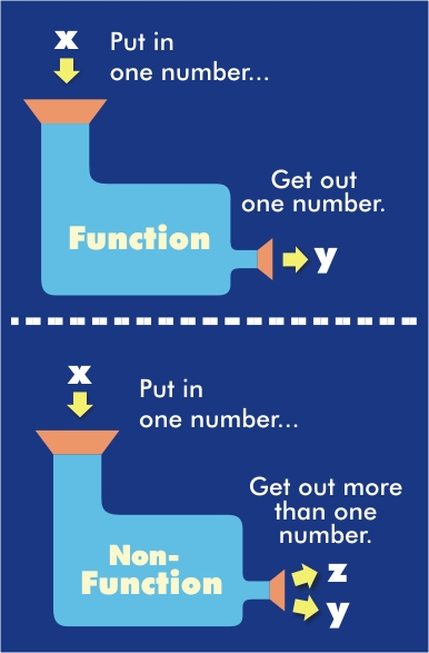
A function is a relation in which each value of the independent variable or domain (usually represented by x) corresponds to exactly one value of the dependent variable or range (usually represented by y). This property of functions is sometimes explained using a "function machine" as illustrated below:
On a graph, the vertical line test can be used to see if a relation has one and only one value of y for each value of x. If no two points on a graph can be joined by a vertical line, the graph represents a function. This is shown in the examples below:
Investigation 2
In Investigation 2, you will explore a new function where the independent variable is an exponent, for example, y = 2x. This type of function is referred to as an exponential function. To crate a table of values of this function, recall the idea of exponents:

Therefore, a partial table of values for ![]() would be
would be
x |
0 |
1 |
2 |
3 |
y |
1 |
2 |
4 |
8 |
The purpose of this investigation is to discover if there is a common ratio between successive y-values for equal increments of x. In other words, is the ratio of successive y-values a constant?
Steps A through E should be very straightforward and pose no serious problems. Be sure to draw these graphs on graph paper as instructed without using technology. Save these in your notebook to refer to later.
Step F is important since it will confirm or deny the relationship regarding common ratios between the successive y-values. It is very important to note that the x-values are incremented by the same amount (in the first case by 2). Unless there are equal x-value increments, the common ratio between successive y-value will not be present.
Investigation Questions
Question 17 on page 115 of your text refers to growth curves and decay curves. For a growth curve, the range values increase for an increase in the domain values. For a decay curve, the range values decrease for an increase in the domain values. This is shown in the diagrams below:
Growth curve Decay curve
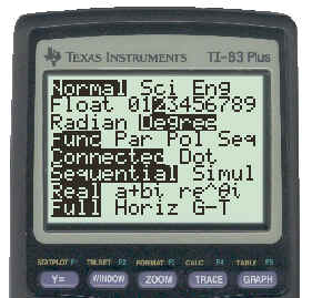
In Investigation Questions 18 and 19, you are asked to draw the tangent to the curve at various places and find their slopes. In the last unit we used the TI83 to do this for us, so you should know how to do it. To make the equation of the tangent more readable, the number of decimal places was fixed at 2 in the [MODE] menu as shown on the screen below. Note that 2 is highlighted in the second row.
The tangent at x = 2.99 for the function y = 2.5x is shown below.
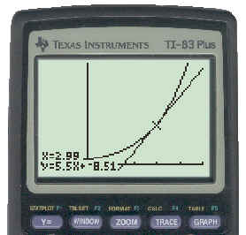
If you want to see the keystrokes necessary to get this curve and tangent click here.
Focus B
Exponential functions are very powerful since they can be used to model many real-world relationships as pointed out in your textbook.
The simplest form of an exponential function is y = bx . Here, b is the base, x is the exponent, and bx is referred to as the power. These functions always pass through the point (0 , 1) because when x = 0, the value of b0 is always 1.
To find the y-value that corresponds to a given x value, it is a simple matter of using the calculator and raising the base to the appropriate exponent. For example, to find y if x = 9 in the equation y = 2x we proceed as follows:
![]()
However, if the y-value is given, it is more difficult to find the corresponding x value. For example, suppose we have to find x if y = 48 in the function ![]() . This means we have to solve an equation that looks like this:
. This means we have to solve an equation that looks like this:![]() .
.
We will discover how to do this algebraically later in this unit, but for now we can use our TI83 calculator to get an approximate solution for us. There are several ways of doing this on the TI83. One is to draw the graph and use [TRACE] and [ZOOM] to get a better and better approximation. Another is to enter the function and use the [TBLSET] and [TABLE] menus to find an approximate value. Again, you refine the table with the starting and increment to get a better and better approximation.
A slicker way is to use the [MATH] an [0:Solver..] menus. To use it we first rearrange the equation we wish to solve and let it equal 0. The above equation becomes:
0 = 2x - 48
Entering this equation, the TI83 produces a solution like the one shown below:
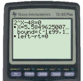
It tells us that x = 5.58 makes the equation true. You can ignore the rest of the stuff on the screen for now. To view the keystrokes for this method click here.
In Unit 1 we learned that to determine if a set of data, which has equal increments in the x values, can be modeled by a linear, quadratic, or higher power function, we check the sequence of differences of the y values.
To determine if a set of data, which has equal increments in the x values, can be modeled by an exponential function, we check the sequence of ratios of successive y-values. This is necessary for answering Question 29 on pages 116 & 117 of your text.
Activity
- Complete Investigation 2 on page114 in your text.
- Complete the Investigation Questions 15 - 21 on page 115.
- Read through Focus B on pages 115 & 116.
- Complete the Focus Questions 22 - 28 on page 116.
- Do the CYU Questions 29 - 33 on pages 116 - 119.
When you have completed these questions, ask your on-site teacher to get the solutions for you from the Teacher's Resource Binder and check them against your answers. After you do this, if there is something you had trouble with and still do not understand, contact your on-line teacher for help.
Test Yourself
- Marcie's father invested $500 for her on the day she was born. The interest on the investment was guaranteed at a rate of 8% and was to be compounded annually (that is, the interest is added to the previous balance at the end of each year and the new amount is then used as the principle for calculating interest in the succeeding year).
(a) Make up a table showing the value of the investment at the end of
each year up until Marcie is 7 years old.
(b) Can the values in the table be represented by an exponential function?
If so is it a growth or decay function?
(c) How much money will she have if she leaves the investment till she is
21?
(d) How long will she have to wait before the investment is at least $5000?